
Introduction
In this blog post, we want to introduce the user to the concept of using Machine Learning techniques designed to originally spot anomalies in written (English) sentences, and instead apply them to support the Threat Analyst in spotting anomalies in security events.
The basic idea behind this is that we try to identify sentences that look “odd” or unusual – but instead of looking at sentences as a sequence of English words, we will look at security event data in order to spot anomalies.
Confused? Let’s look at an example! Similar to how “The cat is barking” is an anomalous English sentence (we wouldn’t expect a cat to bark!), an analyst can visually detect that the process “C:\Users\Public\svchost.exe” runs in a suspicious directory – from the experience of the analyst, the svchost.exe process would never be expected to run from a user’s Public directory – so this is most likely a sample that requires further investigation! The major difference between both use cases is that words in English sentences will become directory and process names in root/process definition – but the core concept of spotting these anomalies remain the same.

Another example of lexical anomalies present in event logs analysis is the appearance of usernames that don’t respect a specific company naming convention.
To illustrate, let’s take the company “NVISO” and two users; “James Smith”, and “Ann-Catherine Jones”, with respectively two different permission levels; “User” and, “Admin”.
If the naming convention is:
<company_name>-<lowercase_first_name_initials><lowercase_familly_name>-<permission_level>
We would have for; “James Smith”, and “Ann-Catherine Jones”, the respective usernames; “NVISO-jsmith-USER”, and “NVISO-acjones-ADMIN”.
Therefore, if all usernames of the company respect that convention and some of them don’t, like “NVIS0–ACJones-admin” or “NVISO-hand3rson-admin”, one can classify them as suspicious users.

Similarly of finding typos in English words, these suspicious users can be spotted by finding the letters/characters that don’t comply the naming convention.
In this article, I will explain how Word2Vec can detect lexical anomalies and how to use it with the our in-house developed open-source framework ee-outliers to detect outliers in Elasticsearch events.
How to find lexical anomalies?
Lexical anomalies can be determined in two dimensions; its wrong syntax and/or its wrong semantics. The term syntax refers to grammatical structure whereas the term semantics refers to the meaning of the vocabulary symbols arranged with that structure.
That’s where Word2Vec comes into play!
Word2Vec
Word2Vec is a highly popular Natural Language Processing model mainly used to produce word embeddings. Word embeddings is the technique that allows you to represent individual words as real-valued vectors in a predefined vector space.
This approach can capture different degrees of similarity between words. In more details, semantic and syntactic patterns can be reproduced using vector arithmetic.
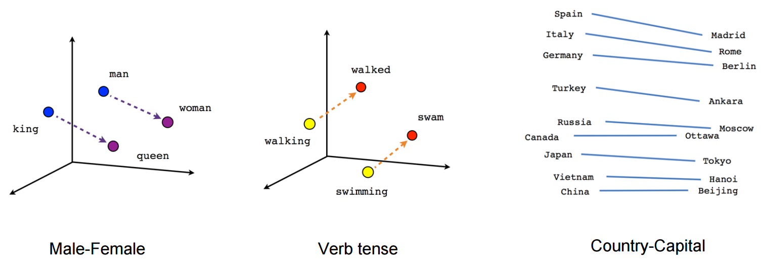
For example, patterns such as “Man is to Woman what King is to Queen” can be – as illustrated in Figure 1- generated through algebraic operations on the vector representations of theses words such that the vector representation of “King” – “Man” + “Woman” produces a result which is closest to the vector representation of “Queen”. Such relationships can be generated for a range of semantic relations (such as Country-Capital) as well as syntactic relations (e.g. Present tense-Past tense).
Word2Vec: Model task
In this demonstration, we chose to use the skip-gram variant of word2vec. This architecture is trained to predict for a given word, named the center word, the words that are likely to surround it, named the context words. For example, if we consider the sentence “The quick brown fox jumped over the lazy dog.”, and a window of size 2 surrounding each center word, we will have the following pairs of (center word, context word):

Now let’s imagine that we have our training documents that contain a vocabulary of 10000 unique words.
To feed the Word2Vec neural network, we will represent the input word like the “ants” as a one-hot vector of size 10000. As illustrated in Figure 3, the one-hot vector of “ants” will have 10000 components (one for every word in our vocabulary) and we’ll place a “1” in the position corresponding to the word “ants”, and “0” in all of the other positions.

If you observe the above figure, you can see that the one-hot vector will then be fed to 2 layers of neurons;
- The first layer of 300 neurons can be represented by a matrix of shape [10000, 300]. It will actually represent the word embeddings of the center words where each row vector represents a center word embedding of size 300 (see Figure 4).
- The second layer of 10000 neurons can be represented by a matrix of shape [300, 10000]. It will represent the word embeddings of the context words where each column vector represents the context word embedding of size 300 (see Figure 4).

Note that the decision of having 300 neurons contained in the first layer is arbitrary. It correspond to the size of the word embeddings and has to be tuned depending of your application. A higher embedding size will increase the computational complexity but also the quality of the model. However, at some point, the marginal quality gain obtained by a higher embedding size will become irrelevant.
The output of the network is, like the input, a single vector of size 10000. This vector contains for every word in our vocabulary, the probability that this word appears given the selected input word (in our case “ants”). The computation of those probabilities will be explained later.
Word2Vec: In detail
Now let’s see in detail how Word2Vec is computing the probability that a context word appears given a certain center word.
As an example, we take the pair (center word, context word) = (“ants”, “car”).
First, as illustrated on Figure 5, the one-hot vector of “ants” will be multiplied by the Center Word Embedding Matrix, which results in a center word embedding vector of “ants”. Note that this operation can be summarised by just taking directly, in the Center Word Embedding Matrix, the row that corresponds to the center word embedding vector of “ants”.

Secondly, as illustrated in Figure 6, the center word embedding vector of “ants” will be multiplied by the Context Word Embedding Matrix. It outputs a vector Xants=[x1,..,xi,..,xn] of size 10000 with values between -inf and +inf. Each of these output values xi (that we are going to call “raw values”) represents the probability that given the word “ants” the word wordi appears. If xi is high compared to the values contained in Xants, it means there is a big probability that given the word “ants”, wordi will appear.

To convert the “raw values” into actual probabilities, the final step is to use a softmax regression. For more information about softmax regression, there is an in-depth tutorial here, but the main idea is to produce an output between 0 and 1 with a sum of all outputs of the same vector equal to 1.
Therefore, if we for example want to know the probability for the pair (center word, context word) = (“ants”, “car”) we will have to calculate excar/sum(eXants). Note that Xants=[x1,..,xi,..,xcar,..,xn] is a vector when xcar is the “raw value” contained in Xants corresponding to the word “car”. This operation is illustrated on Figure 7.

Now that we have our probabilities for each (center word, context word) pair, we can actually assign a score to each word depending on their surrounding words.
Assigning a score for each word
If you observe Table 1, you can notice that when analysing one example phrase, multiple probabilities are related to each unique word. Without having a unique score for each word, it becomes hard to evaluate if one of these words can be considered anomalous or not. This is because a simple probability, which is the relation between just two words, doesn’t provide enough information about the context.
Therefore, we do need to perform some additional operations to assign each word a unique score.
| Center words | Context words | Probabilities |
|---|---|---|
| C: | parent_directory | P1 |
| C: | sub_directory | P2 |
| parent_directory | C: | P3 |
| parent_directory | sub_directory | P4 |
| parent_directory | sub_sub_directory | P5 |
| sub_directory | C: | P6 |
| sub_directory | parent_directory | P7 |
| sub_directory | sub_sub_directory | P8 |
| sub_directory | process.exe | P9 |
| sub_sub_directory | parent_directory | P10 |
| … | … | … |
For that purpose, we developed 3 types of score:
- Center Word Score: If this score is high/low, it means that this word often/rarely sees the current context words.
- Context Word Score: If this score is high/low, it means that this word is often/rarely observed by the current context words.
- Total Word Score: Combination of both center- and context- word scores. Therefore, if a word score is low, it means that this word rarely sees and/or is rarely observed by the context words.
Center Word Score computation
The center word score is calculated by using the geometric mean of all the probabilities corresponding to the current word as a center word. If we take the example on Table 1, we will then compute the center word score of the word sub_directory as follow:
cntr_scr_sub_directory = (P6*P7*P8*P9)1/4
Context Word Score computation
For the context word score, we do the opposite, we calculate it by using the geometric mean of all the probabilities corresponding to the current word as a context word. If we take the example on Table 1, we will compute the context word score of the word parent_directory as follow:
cntxt_scr_parent_directory = (P1*P7*P10)1/3
Total Word Score computation
The Total Word Score is simply the geometric mean between the Center Word Score and the Context Word Score. Therefore the total word score of the word sub_directory can be computed as follow:
ttl_scr_sub_directory = (cntr_scr_sub_directory*cntxt_scr_sub_directory)1/2
Outlier Detection Methods
If we made the efforts to assign a score for each word, it is to reaching our main objective of spotting anomalies/outliers. We started with the assumption that words contained in texts should have similar context/neighbourhood words. Therefore, if semantic and syntactic rules are respected, we will expect for each unique word a similar score each time it will appear. In contrast, if semantic and syntactic rules are not respected in the neighbourhood of a center word, the score should be lower and very different compared to the score of that word in normal context. Therefore, the distribution of the score of each word could look like this:

Taking this assumption, we can then spot outliers, for example, using the Standard Deviation Method and selecting outliers as follow:
if word_score < (mean_score - X*stdev_score):
     is_outlier = True
Where:
word_scoreis the score ofwordiintexti.mean_scorethe mean of the scores ofwordiin all texts.Xis thetrigger_sensitivity.stdev_scoreis the standard deviation of the scores ofwordiin all texts.
Note that you can use other basic statistic methods like Interquartile Range Method (IQD) or the Median Absolute Deviation Method (MAD).
using Word2Vec with ee-outliers to detect anomalies in Elasticsearch events
ee-outliers is an open-source framework we developed to detect outliers in Elasticsearch events. In this section, I will dive into how you can use Word2Vec with ee-outliers for your own security monitoring activities.
In this small tutorial, we will see how the Word2Vec analyzer from ee-outliers can detect abnormal usernames. Abnormal usernames can vary in shapes. While the obvious random names are easy to spot, users created by adversaries leverage a multitude of mechanisms to stay covert such as character substitution.
Let’s get started!
Preparing the data
For test purposes, I decided to generate a synthesised dateset containing 10000 “normal” usernames that respect the following structure:
NVISO-<lowercase_first_name_initials><lowercase_family_name>-<permission_level>
And create 50 “suspicious” usernames that are based on that structure but with 2 letters switched with a random character.

The used dataset is available here in CSV format. Note that, to make it work with ee-outliers, I assigned different timestamps to each of the usernames. I also added a special column named “label” set to 0 for normal and 1 for suspicious events.
You can upload the dataset to Elasticsearch by using Kibana. From the home menu, in the section “Upload data from log file”, simply click on “Import a CSV, NDJSON, or log file” and follow the instructions by keeping the default parameters and naming the index generated_usernames.
Preparing ee-outliers
The Getting started section on GitHub contains all the information to correctly set-up ee-outliers. Concerning the default configuration file, you will have to only modify the following parameters:
es_index_pattern: Has to be set to the Elasticsearch index namegenerated_usernamesthat you created earlier.history_window_days: Specify how many days back in time to process events and search for outliers. Has the synthesised dataset has been set with a static timestamp we recommend you to put a high history window like600days to be sure of catching all events.
In the next section, we will focus on building a detection use case using Word2Vec.
Creating a new use case
For the detection use case, you will have to create an independent configuration file in the directory use_cases/examples and name it word2vec_suspicious_username.conf.
After, you can define the use case as follow:
##############################
# WORD2VEC - SUSPICIOUS USERNAME
##############################
[word2vec_suspicious_username]
es_query_filter=username: *
target=username
aggregator=aggr

word2vec_batch_eval_size=3400
min_target_buckets = 1000

use_prob_model=0

separators=""
size_window=1
num_epochs=2
learning_rate=0.001
embedding_size=20
seed=42

# Print outlier scores on standard output.
print_score_table=1
# Print confusion matrix and precision, recall and F-Measure metrics on standard output.
print_confusion_matrix=1

trigger_focus=word
trigger_score=center

trigger_on=low
trigger_method=stdev
trigger_sensitivity=3.2

outlier_type=suspicious user activity
outlier_reason=suspicious username detected
outlier_summary=suspicious username detected: {username}

run_model=1
test_model=0
The use case can be explained as follows:
- The
es_query_filterselects all Elasticsearch events that contain ausernamefield. - The event field(s) specified in
targetwill be selected and gather in batches of sizeword2vec_batch_eval_size. It defines how many events should be processed at the same time, before looking for outliers. Bigger batches means better results but increased memory usage. - Then the
targetelement(s) will be spit by the occurrence of regex pattern defined inseparators. In other words, it will split the text contained in thetargetelements by words. In our example, if the text is “NVISO-mroberti-users”, withseparators="", the split in words will look like: [N, V, I, S, O, -, m, r, o, b, …]. - The
size_windowis the size of the window illustrated in Figure 2 which determines how pairs of (center word, context word) are done. - After, the pairs of (center word, context word) will be fed to the Word2Vec model. This action is divided into two phases; training & evaluation. During the training phase, the entire batch of target data will pass
num_epochstimes through word2vec and be trained with backpropagation and alearning_rateequal to0.001. The evaluation phase will then just pass all the data through the Word2Vec model and output the probabilities linked to each pair (center word, context word). - Finally, as
trigger_scoreis set tocenter, a center score is computed for each word. It will then, use the Standard Deviationtrigger_methodwith atrigger_sensitivityof 3.2 to spot words considered as outliers. Note that if one word is considered as an outlier, the algorithm will consider the entire text element as an outlier.
For information about parameters not mentioned in this example, you can consult the “All parameters in configurations” section on GitHub.
Running ee-outliers
Details on how to deploy the use case we just constructed in ee-outliers can be found in the documentation.
If you did everything right, ee-outliers should run and finish with on the standard output something similar to this:
outliers | 2020-06-10 13:46:55 - INFO - =======c=====================
outliers | 2020-06-10 13:46:55 - INFO - ===== analysis summary =====
outliers | 2020-06-10 13:46:55 - INFO - ============================
outliers | 2020-06-10 13:46:55 - INFO - total use cases processed: 7
outliers | 2020-06-10 13:46:55 - INFO - total outliers detected: 45
outliers | 2020-06-10 13:46:55 - INFO - total whitelisted outliers: 0
outliers | 2020-06-10 13:46:55 - INFO -
outliers | 2020-06-10 13:46:55 - INFO - succesfully analyzed use cases: 7
outliers | 2020-06-10 13:46:55 - INFO - succesfully analyzed use cases without events: 6
outliers | 2020-06-10 13:46:55 - INFO - succesfully analyzed use cases with events: 1
outliers | 2020-06-10 13:46:55 - INFO -
outliers | 2020-06-10 13:46:55 - INFO - use cases skipped because of missing index: 0
outliers | 2020-06-10 13:46:55 - INFO - use cases skipped because of incorrect configuration: 0
outliers | 2020-06-10 13:46:55 - INFO - use cases that caused an error: 0
outliers | 2020-06-10 13:46:55 - INFO -
outliers | 2020-06-10 13:46:55 - INFO - total analysis time: 0d 0h 0m 6s
outliers | 2020-06-10 13:46:55 - INFO - average analysis time: 0d 0h 0m 6s
outliers | 2020-06-10 13:46:55 - INFO -
outliers | 2020-06-10 13:46:55 - INFO - most time consuming use cases (top 10):
outliers | 2020-06-10 13:46:55 - INFO -      + word2vec_suspicious_username - 10,050 events - 45 outliers - 0d 0h 0m 6s
outliers | 2020-06-10 13:46:55 - INFO - ============================
outliers | 2020-06-10 13:46:55 - INFO - asking housekeeping jobs to shutdown after finishing
outliers | 2020-06-10 13:46:55 - INFO - housekeeping thread #140414014527232 stopped
outliers | 2020-06-10 13:46:55 - INFO - finished performing outlier detection
outliers exited with code 0
Result analysis
In this dataset configuration, all events classified as outliers – the usernames that don’t respect the convention – are gathered in the same window of time. It is done in a way that if we chronologically analyse the dataset of size 10050, with batches of size 3400, we will have all the outliers gathered in the first batch. It’s a good practice to see if it first detect a large number of outliers in a dataset full of outliers – and secondly if it doesn’t create false positives when there is no outlier contained in the dataset.
Let’s now analyse our results!
With the same parameters defined in the use case above, we obtain for the first batch the following confusion matrix and metric scores;

We can see that it worked pretty well! 46 of the 50 outliers have been found, and no False Positives have been created, which result in a F-Score of 0.96!
Now let’s look at confusion matrices of the 2 next batches that contain no outliers:


Unfortunately, the third and last batch catched a False Positive. Taking a look in detail at its table score can help us to find out a potential reason why it has been misclassified as an outlier.

If we observe Figure 8, we can see that there is something wrong around the character “-“. What that low score means, is that given the character “-” there is a low probability to have the character “x” and “A” around it. “-” and “A” are mostly appearing just after the end of the family name (<lowercase_family_name>-ADMIN). Therefore, we can conclude that within the third batch not a lot of family names are ending by “x”.
If you now play a bit with the trigger_sensitivity parameter, you will see that the more you decrease/increase and the more the number of FP and TP will grow/drop.
Note that the confusion matrix and f-score can be printed only if your Elasticsearch dataset is labeled by a special field named “label” where non-anomalous and anomalous events are respectively set to 0 and 1.
Elasticsearch event tagging
If in your general configuration file the parameter es_save_results is set to 1, all the events considered as outliers will be tagged with a range of new fields, all prefixed with outliers.<outlier_field_name>. On Figure 9, you can see that those extra fields contain information like:
outliers.model_type: The type of analyser used. In this case,word2vecbut can beterms,metricsorsimplequery.outliers.size_window: size of the word2vec window.outliers.score_type: The type of word score used. Can becenter,context, ortotal.outliers.expected_window_words: The most expected words in the window the outlier characters.outliers.expected_words: The most expected word in place of the outlier character.outliers.score: The score of each outlier word/character.outliers.decision_frontier: The decision frontier of each outlier word/character.outliers.confidence: The confidence corresponds to the absolute difference between the outlier word/character score and his decision frontier.

Conclusion
We created a model based on Word2Vec which allows us to detect outliers/anomalies within text respecting specific syntactic and semantic rules.
A small demonstration and analysis show us the real potential of Word2Vec. In some cases, it can detect a large number of outliers while keeping the number of False Positive down.
This algorithm is still in a Beta state and we look forward to seeing how it holds up in other use cases. We are also impatient to see the community (maybe you) using it and giving some feedback!
I hope you enjoyed the article and found it useful. Thanks for reading and don’t hesitate to leave questions or suggestions – here or in the issue tracker on github.
I will keep writing articles combining Cyber Security and Machine Learning so stay tuned!
Additional content
If you want to know more about how to use ee-outliers with other examples use-cases, I suggest you to read “TLS beaconing detection using ee-outliers and Elasticsearch” or “Detecting suspicious child processes using ee-outliers and Elasticsearch“.
About the author
Maximilien Roberti is a Machine Learning engineer working full-time in the NVISO Labs team. He focuses on building new and exciting models to help the blue teams spot adversaries as part of NVISO’s Threat Hunting and Security Monitoring activities. You can get in touch with Maximilien on LinkedIn or Twitter.
2 thoughts on “Using Word2Vec to spot anomalies while Threat Hunting using ee-outliers”
Comments are closed.